


 14 / 21

u
0
|
r
=
R
=
1
60Δ
[10
T
−
6
−
72
T
−
5
+
+225
T
−
4
−
400
T
−
3
+ 450
T
−
2
−
360
T
−
1
+ 147
E
] +
Δ
6
7
u
VII
;
u
0
|
r
=
R
−
δ
=
1
60Δ
[12
T
5
−
75
T
4
+200
T
3
−
300
T
2
+300
T
1
−
137
E
] +
Δ
5
6
u
VI
;
u
0
|
r
=
R
−
δ
=
1
60Δ
[
−
10
T
6
+ 72
T
5
−
−
225
T
4
+ 400
T
3
−
450
T
2
+ 360
T
1
−
147
E
] +
Δ
6
7
u
VII
.
The main results of computation.
The research computation was
performed using the computing methods developed for experimental
conditions (see Table 1) implemented in a one-diaphragm aerodynamic
shock tube (at the Institute for Problem Mechanics, RAS) [8, 9]. During
the experiments on the shock tube mentioned above, which were then
subjected to the numerical analysis, at the initial instant of time (i.e., before
the rupture of the diaphragm), the low pressure chamber (LP chamber)
was filled with air (test gas) at pressure
p
LP c
[mbar] and temperature
T
= 298
.
15
K, while the high pressure chamber (HP chamber) was
filled with a compressed air at pressure
P
HP c
[mbar] and temperature
T
= 298
.
15
K. The experimental facility at the Institute for Applied
Mechanics, RAS, looks like a tube of an uniform cross-section (internal
diameter
D
= 0
.
8
m; length of low pressure chamber
L
LP c
= 7
.
35
m;
length of high pressure chamber
L
HP c
= 1
.
97
m) and is designed for the
value range of Mach numbers SW
M
= 6
. . .
12]
.
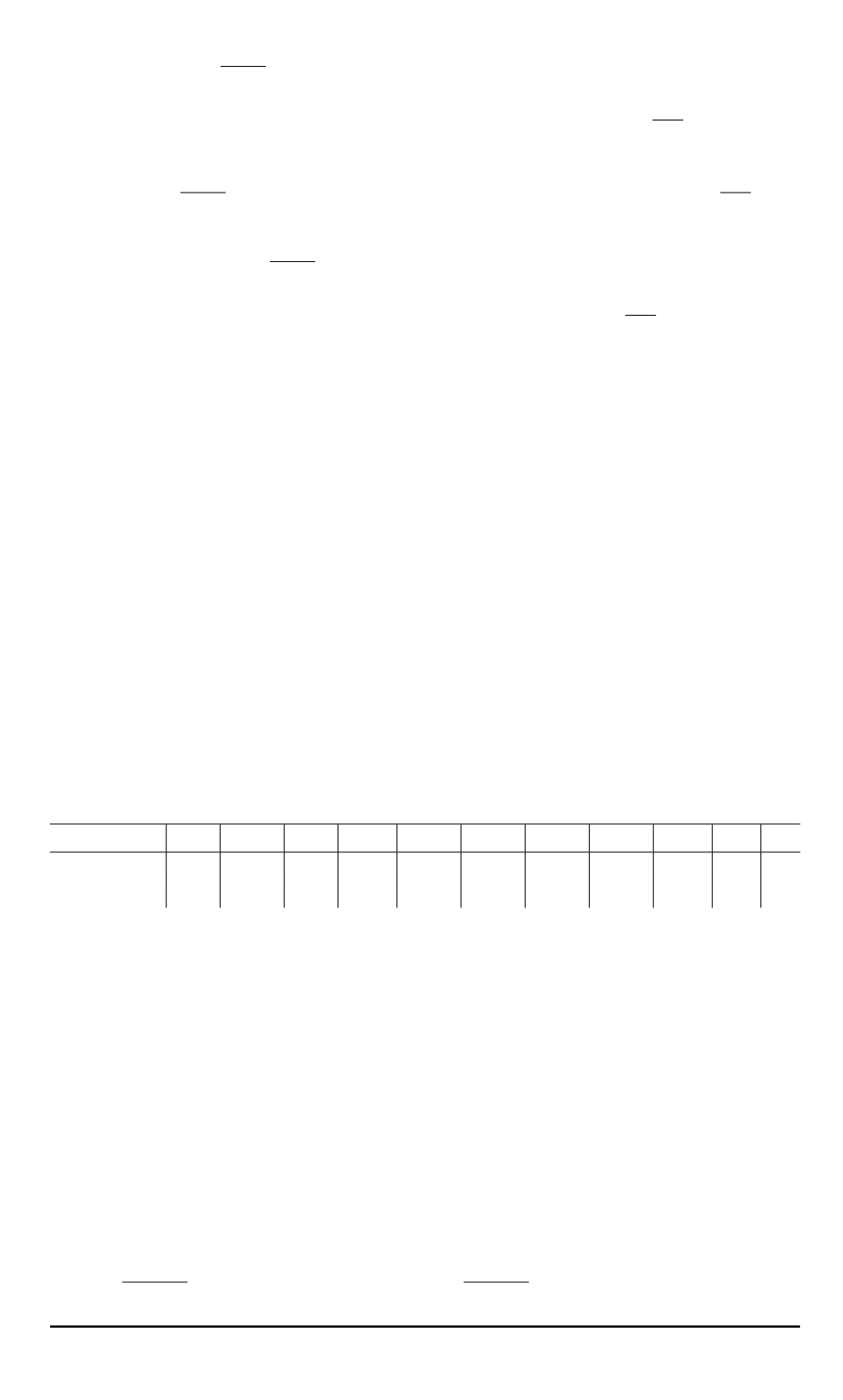
No
1 2 3 4 5
6
7
8 9 10 11
p
HPc
, atm 10 10.2 22 19 13.2 19.5 19.5 20.5 21 36 34
p
LPc
, atm 0.3 15 6.6 100 2 0.7 5.6 100 100 1 1
In Fig. 2, the layout chart of the pressure gauge locations used for
obtaining the experimental time dependences of pressure
P
(
t
)
(in different
spatial points) is shown.
In Fig. 3, the experimental (Experiment 4) time dependencies of
pressure
P
(
t
)
for the second and third pressure gauges are shown (pressure
gauge 1 is at the right end of the shock tube plane (the Institute of Problem
Mechanics, RAS, see Fig. 2.)
From the graphs in Fig. 3, it follows that only gas-dynamic parameters
can be evaluated (by the times of the shock wave arrivals to the pressure
gauges) behind the front of the initial shock wave (gauge 2:
z
= 5
.
78
m,
t
= 8
.
92
ms; gauge 3:
z
= 9
.
22
m,
t
= 14
ms):
D
SW
≈
0
.
7
km/s,
u
2
=
2
γ
1
+ 1
D
SW
≈
0
.
6
km/s,
p
2
=
2
γ
1
+ 1
ρ
1
D
2
SW
≈
0
.
5
atm. From
16 ISSN 0236-3941. HERALD of the BMSTU. Series “Mechanical Engineering”. 2014. No. 1